14 The Need for Optimization

Only once we have a solid characterization of the surface area we want to improve can we begin to identify the best way to improve it.

Refactoring at Scale (Lemaire 2020)

14.1 Build first, then optimize

14.1.1 Identifying bottlenecks

Refactoring existing code for speed sounds like an appealing activity for a lot of us: it is always satisfying to watch our functions get faster, or finding a more elegant way to solve a problem that also results in making your code a little bit faster. Or as Maude Lemaire writes in Refactoring at Scale (Lemaire 2020), “Refactoring can be a little bit like eating brownies: the first few bites are delicious, making it easy to get carried away and accidentally eat an entire dozen. When you’ve taken your last bite, a bit of regret and perhaps a twinge of nausea kick in.”

But beware! As Donald Knuth puts it “Premature optimization is the root of all evil”. What does that mean? That focusing on optimizing small portions of your app before making it work fully is the best way to lose time along the way, even more in the context of a production application, where there are deadlines and a limited amount of time to build the application. Why? Here is the general idea: let’s say the schema in Figure 14.1 represents your software, and its goal is to make things travel from X1 to X2, but you have a bottleneck at U. You are building elements piece by piece: first, the portion X1.1 of the “road”, then X1.2, etc. Only when you have your application ready can you really appreciate where your bottleneck is, and you can focus on making things go fast from X1.1 to X.1.2, these performance gains won’t make your application go faster: you will only make the elements move faster to the bottleneck.

When? Once the application is ready: here in our example, we can only detect the bottleneck once the full road is actually built, not while we are building the circle.

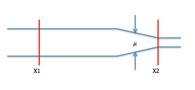
FIGURE 14.1: Road bottleneck, from WikiMedia https://commons.wikimedia.org/wiki/File:Roadway_section_with_bottleneck.png.

This bottleneck is the very thing you should be optimizing: having faster code anywhere else except this bottleneck will not make your app faster: you will just make your app reach the bottleneck faster, but there will still be this part of your app that slows everything down. But this is something you might only realize when the app is fully built: pieces might be fast individually, but slow when put together. It is also possible that the test dataset you have been using from the start works just fine, but when you try your app with a bigger, more realistic dataset, the application is actually way slower than it should be. And, maybe you have been using an example dataset so that you do not have to query the database every time you implement a new feature, but the SQL query to the database is actually very slow. This is something you will discover only when the application is fully functional, not when building the parts, and realizing that when you only have 5% of the allocated time for this project left on your calendar is not a good surprise.

Or to sum up:

Get your design right with an un-optimized, slow, memory-intensive implementation before you try to tune. Then, tune systematically, looking for the places where you can buy big performance wins with the smallest possible increases in local complexity.

The Art of UNIX Programming (Raymond 2003)

14.1.2 Do you need faster functions?

Optimizing an app is a matter of trade-offs: of course, in a perfect world, every piece of the app would be tailored to be fast, easy to maintain, and elegant. But in the real world, you have deadlines, limited time and resources, and we are all but humans. That means that at the end of the day, your app will not be completely perfect: software can always be made better. No piece of code has ever reached complete perfection.

Given that, do you want to spend 5 days out of the 30 you have planned optimizing a function so that it runs in a quarter of a second instead of half a second, then realize the critical bottleneck of your app is actually the SQL query and not the data manipulation? Of course a function running twice as fast is a good thing, but think about it in context: for example, how many times is this function called? We can safely bet that if your function is only called once, working on making it twice as fast might not be the one function you would want to focus on (well, unless you have unlimited time to work on your project, and in that case lucky you; you can spend a massive amount of time building the perfect software). On the other hand, the function which is called thousands of times in your application might benefit from being optimized.

And all of this is basic maths. Let’s assume the following:

A current scenario takes 300 seconds to be accomplished on your application.
One function A() takes 30 seconds, and it’s called once.
One function B() takes 1 second, and it’s called 50 times.

If you divide the execution time of A() by two, you would be performing a local optimization of 15 seconds, and a global optimization of 15 seconds. On the other hand, if you divide the execution time of B() by two, you would be performing a local optimization of 0.5 seconds, but a global optimization of 25 seconds.

Again, this kind of optimization is hard to detect until the app is functional. An optimization of 15 seconds is way greater than an optimization of 0.5 seconds. Yet you will only realize that once the application is up and running!

14.1.3 Don’t sacrifice readability

As said in the last section, every piece of code can be rewritten to be faster, either from R to R or using a lower-level language: for example C or C++. You can also rebuild data manipulation code switching from one package to another, or use a complex data structures to optimize memory usage, etc.

But that comes with a price: not keeping things simple for the sake of local optimization makes maintenance harder, even more if you are using a lesser-known language/package. Refactoring a piece of code is better done when you keep in mind that “the primary goal should be to produce human-friendly code, even at the cost of your original design. If the laser focus is on the solution rather than the process, there’s a greater chance your application will end up more contrived and complicated than it was in the first place” (Lemaire 2020).

For example, switching some portions of your code to C++ implies that you might be the only person who can maintain that specific portion of code, or that your colleague taking over the project will have to spend hours learning the tools you have been building, or the language you have chosen to write your functions with.

Again, optimization is always a matter of trade-off: is the half-second local optimization worth the extra hours you will have to spend correcting bugs when the app will crash and when you will be the only one able to correct it? Also, are the extra hours/days spent rewriting a working code-base worth the speed gain of 0.5 seconds on one function?

For example, let’s compare both these implementations of the same function, one in R, and one in C++ via Rcpp (Eddelbuettel et al. 2023). Of course, the C++ function is faster than the R one—this is the very reason for using C++ with R.

library("Rcpp")
# A C++ function to compute the mean
cppFunction("
double mean_cpp(NumericVector x) {
  int j;
  int size = x.size();
  double res = 0;
  for (j = 0; j < size; j++){
    res = res + x[j];
  }
  return res / size;
}")

# Computing the mean using base R and C++, 
# and comparing the time spent on each
benched <- bench::mark(
  cpp = mean_cpp(1:100000),
  native = mean(1:100000), 
  iterations = 1000
)
benched

# A tibble: 2 × 6
  expression    min median `itr/sec` mem_alloc `gc/sec`
  <bch:expr> <bch:> <bch:>     <dbl> <bch:byt>    <dbl>
1 cpp         152µs  154µs     5316.     784KB     21.3
2 native      692µs  701µs     1422.        0B      0

(Note: we will come back to bench::mark() later.)

However, how much is a time gain worth if you are not sure you can get someone on your team to take over the maintenance if needed? In other words, given that (in our example) we are gaining around -5.4654^{-4} on the execution time of our function, is it worth switching to C++? Using external languages or complex data structures implies that from the start, you will need to think about who and how your codebase will be maintained over the years.

Chances are that if you plan on using a shiny application during a span of several years, various R developers will be working on the project, and including C++ code inside your application means that these future developers will either be required to know C++, or they will not be able to maintain this piece of code.

So, to sum up, there are three ways to optimize your application and R code, and the bad news is that you cannot optimize for all of them:

Optimizing for speed
Optimizing for memory
Optimizing for readability/maintainability

Leading a successful project means that you should, as much as possible, find the perfect balance between these three.

14.2 Tools for profiling

14.2.1 Profiling R code

A. Identifying bottlenecks

The best way to profile R code is by using the profvis (Chang, Luraschi, and Mastny 2020) package,⁵³ a package designed to evaluate how much time each part of a function call takes. With profvis, you can spot the bottleneck in your function. Without an automated tool to do the profiling, the developers would have to profile by guessing, which will, most of the time, come with bad results:

One of the lessons that the original Unix programmers learned early is that intuition is a poor guide to where the bottlenecks are, even for one who knows the code in question intimately.

The Art of UNIX Programming (Raymond 2003)

Instead of guessing, it is a safe bet to go for a tool like profvis, which allows you to have a detailed view of what takes a long time to run in your R code.

Using this package is quite straightforward: put the code you want to benchmark inside the profvis() function,⁵⁴ wait for the code to run, and that is it; you now have an analysis of your code running time.

Here is an example with 3 nested functions, top(), middle() and bottom(), where top() calls middle() which calls bottom():

library(profvis)
top <- function(){
  # We use profvis::pause() because Sys.sleep() doesn't 
  # show in the flame graph
  pause(0.1)
  # Running a series of function with lapply()
  lapply(1:10, function(x){
    x * 10
  })
  # Calling a lower level function
  middle()
}

middle <- function(){
  # Pausing before computing, and calling other functions
  pause(0.2)
  1e4 * 9
  bottom_a()
  bottom_b()
}

# Both will pause and print, _a for 0.5 seconds, 
# _b for 2 seconds
bottom_a <- function(){
  pause(0.5)
  print("hey")
}
bottom_b <- function(){
  pause(2)
  print("hey")
}
profvis({
  top()
})

What you see now is called a flame graph: it is a detailed timing of how your function has run, with a clear decomposition of the call stack. What you see in the top window is the expression evaluated, and on the bottom the details of the call stack, with what looks a little bit like a Gantt diagram. This result reads as follow: the wider the function call, the more time it has taken R to compute this piece of code. On the very bottom, the “top” function (i.e. the function which is directly called in the console), and the higher you go, the more you enter the nested function calls.

Here is how to read the graph in 14.2:

On the x axis is the time spent computing the whole function. Our top() function being the only one executed, it takes the whole record time.
Then, the second line shows the functions which are called inside top(). First, R pauses, then does a series of calls to FUN (which is the internal anonymous function from lapply()), and then calls the middle() function.
Then, the third line details the calls made by middle(), which pauses, then calls bottom_a() and bottom_b(), which each pause() for a given amount of time.

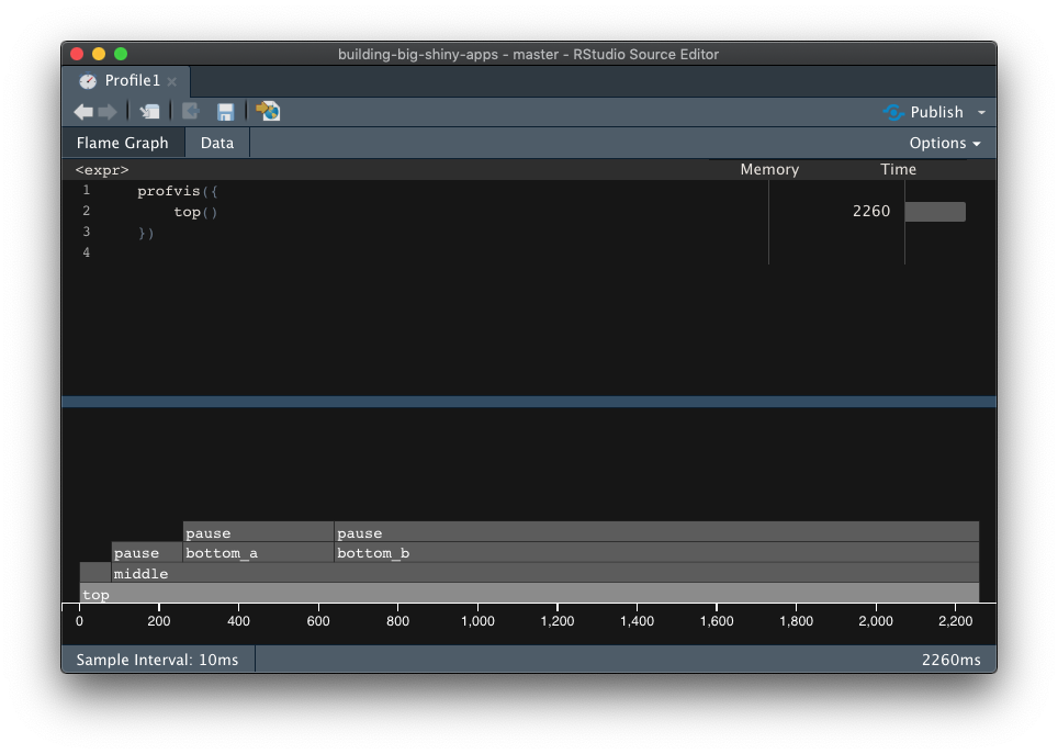
FIGURE 14.2: profvis flame graph.

If you click on the “Data” tab, you will also find another view of the flame graph, shown in 14.3, where you can read the hierarchy of calls and the time and memory spent on each function call:

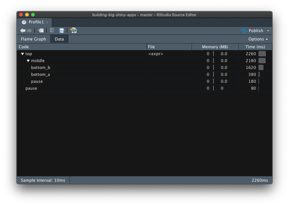
FIGURE 14.3: profvis data tab.

If you are working on profiling the memory usage, you can also use the profmem (Bengtsson 2020) package which, instead of focusing on execution time, will record the memory usage of calls.

library(profmem)
# Computing the memory used by each c
p <- profmem({
  x <- raw(1000)
  A <- matrix(rnorm(100), ncol = 10)
})
p

Rprofmem memory profiling of:
{
    x <- raw(1000)
    A <- matrix(rnorm(100), ncol = 10)
}

Memory allocations:
       what bytes               calls
1     alloc  1048               raw()
2     alloc   280            matrix()
3     alloc   560            matrix()
4     alloc   560            matrix()
5     alloc  1072            matrix()
6     alloc   848 matrix() -> rnorm()
7     alloc  2552 matrix() -> rnorm()
8     alloc   848            matrix()
9     alloc   528          <internal>
10    alloc  1648          <internal>
11    alloc  1648          <internal>
12    alloc  1072          <internal>
13    alloc   256          <internal>
14    alloc   456          <internal>
15    alloc   216          <internal>
16    alloc   256          <internal>
total       13848

You can also get the total allocated memory with:

total(p)

[1] 13848

And extract specific values based on the memory allocation:

p2 <- subset(p, bytes > 1000)
print(p2)

Rprofmem memory profiling of:
{
    x <- raw(1000)
    A <- matrix(rnorm(100), ncol = 10)
}

Memory allocations:
       what bytes               calls
1     alloc  1048               raw()
5     alloc  1072            matrix()
7     alloc  2552 matrix() -> rnorm()
10    alloc  1648          <internal>
11    alloc  1648          <internal>
12    alloc  1072          <internal>
total        9040

(Example extracted from profmem help page).

Here it is; now you have a tool to identify bottlenecks!

B. Benchmarking R code

Identifying bottlenecks is a start, but what to do now? In the next chapter about optimization, we will dive deeper into common strategies for optimizing R and shiny code. But before that, remember this rule: never start optimizing if you cannot benchmark this optimization. Why? Because developers are not perfect at identifying bottlenecks and estimating if something is faster or not, and some optimization methods might lead to slower code. Of course, most of the time they will not, but in some cases adopting optimization methods leads to writing slower code, because we have missed a bottleneck in our new code. And of course, without a clear documentation of what we are doing, we will be missing it, relying only on our intuition as a rough guess of speed gain.

In other words, if you want to be sure that you are actually optimizing, be sure that you have a basis for comparison.

How to do that? One thing that can be done is to keep an RMarkdown file with your starting point: use this notebook to keep track of what you are doing, by noting where you are starting from (i.e, what’s the original function you want to optimize), and compare it with the new one. By using an Rmd, you can document the strategies you have been using to optimize the code, e.ga: “switched from for loop to vectorize function”, “changed from x to y”, etc. This will also be helpful for the future: either for you in other projects (you can get back to this document), or for other developers, as it will explain why specific decisions have been made.

To do the timing computation, you can use the bench (Hester and Vaughan 2021) package, which compares the execution time (and other metrics) of two functions. This function takes a series of named elements, each containing an R expression that will be timed. Note that by default, the mark() function compares the output of each function,

Once the timing is done, you will get a data.frame with various metrics about the benchmark.

# Multiplying each element of a vector going from 1 to size
# with a for loop 
for_loop <- function(size){
  res <- numeric(size)
  for (i in 1:size){
    res[i] <- i * 10
  }
  return(res)
}
# Doing the same thing using a vectorized function
vectorized <- function(size){
  (1:size) * 10
}
res <- bench::mark(
  for_loop = for_loop(1000), 
  vectorized = vectorized(1000), 
  iterations = 1000
)
res

# A tibble: 2 × 6
  expression      min   median `itr/sec` mem_alloc
  <bch:expr> <bch:tm> <bch:tm>     <dbl> <bch:byt>
1 for_loop    42.87µs  43.58µs    22819.    32.4KB
2 vectorized   2.09µs   2.41µs   230412.    11.8KB
# ℹ 1 more variable: `gc/sec` <dbl>

Here, we have an empirical evidence that one code is faster than the other: by benchmarking the speed of our code, we are able to determine which function is the fastest.

If you want a graphical analysis, bench comes with an autoplot method for ggplot2 (Wickham, Chang, et al. 2023), as shown in Figure 14.4:

ggplot2::autoplot(res)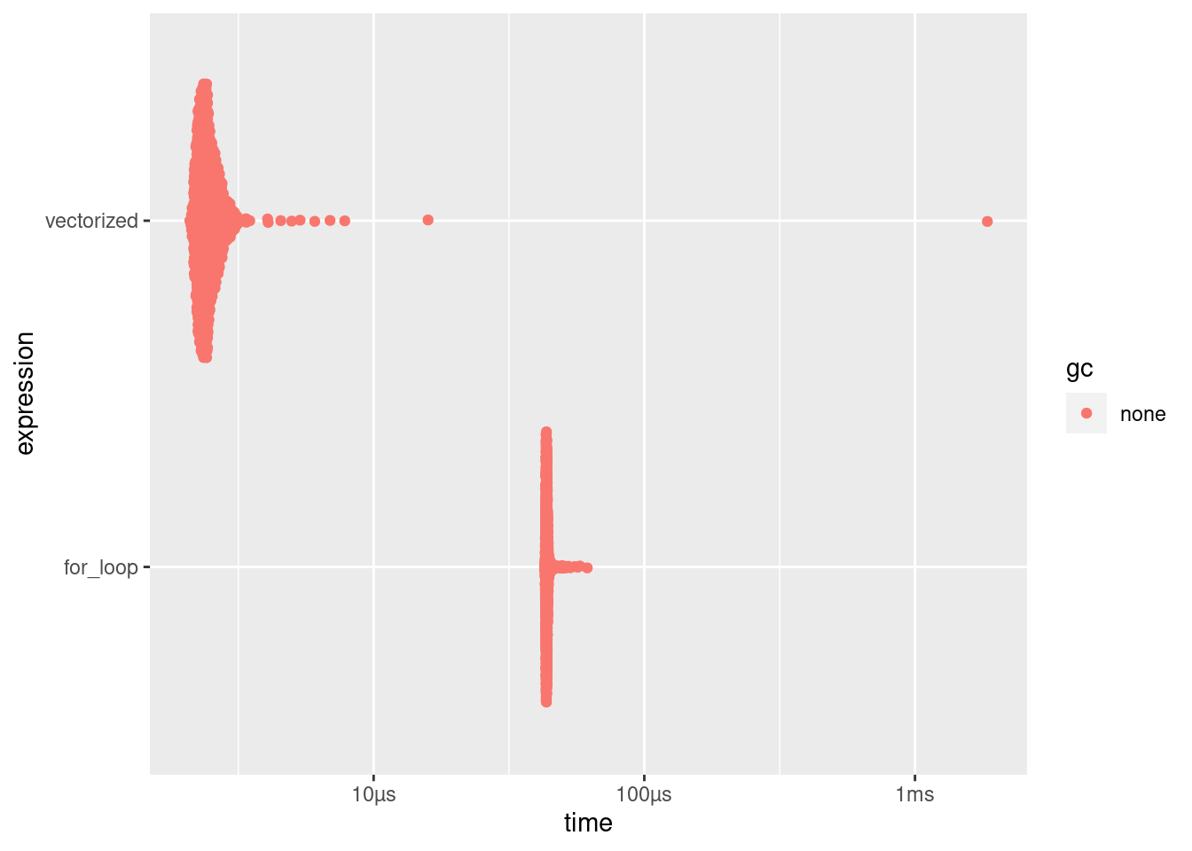

FIGURE 14.4: bench autoplot.

And, bonus point, bench takes time to check that the two outputs are the same, so that you are sure you are comparing the very same thing, which is another crucial aspect of benchmarking: be sure you are not comparing apples with oranges!

14.2.2 Profiling `{shiny}`

A. `{shiny}` back-end

You can profile shiny applications using the profvis package, just as any other piece of R code. The only thing to note is that if you want to use this function with an app built with golem (Fay, Guyader, Rochette, et al. 2023), you will have to wrap the run_app() function in a print() function. Long story short, what makes the app run is not the function itself, but the printing of the function, so the object returned by run_app() itself cannot be profiled. See the discussion of this issue on the {golem} repository to learn more about this.

B. `{shiny}` front-end

Google Lighthouse

One other thing that can be optimized when it comes to the user interface is the web page rendering performance. To do that, we can use standard web development tools: as said several times, a shiny application IS a web application, so tools that are language agnostic will work with shiny. There are thousands of tools available to do exactly that, and going through all of them would probably not make a lot of sense.

Let’s focus on getting started with a basic but powerful tool, that comes for free inside your browser: Google Lighthouse, one of the famous tools for profiling web pages, is bundled into recent versions of Google Chrome. The nice thing is that this tool not only covers what you see (i.e. not only what you are actually rendering on your personal computer), but can also audit your app with various configurations, notably on mobile, with low bandwidth and/or mimicking a 3G connection. Being able to perform an audit of our application as seen on a mobile device is a real strength: we are developing an application on our computer, and might not be regularly checking how our application is performing on a mobile. Yet a large portion of web navigation is performed on a mobile or tablet.

Already in 2016, Google wrote that “More than half of all web traffic now comes from smartphones and tablets”. Knowing the exact number of visitors that browse through mobile is hard: the web is vast, and not all websites record the traffic they receive. Yet many, if not all, studies of how the web is browsed report the same results: more traffic is created via mobile than via computer.⁵⁵

And, the advantages of running it in your browser is that it can perform the analysis on locally deployed applications: in other words, you can launch your shiny application in your R console, open the app in Google Chrome, and run the audit. A lot of online services need a URL to do the audit!

Each result from the audit comes with advice and changes you can make to your application to make it better, with links to know more about the specific issue.

And of course, last but not least, you also get the results of the metrics you have “passed”. It is always a good mood booster to see our app passing some audited points!

Here is a quick introduction to this tool:

Open Chrome in incognito mode (File > New Icognito Window),⁵⁶ so that the page performance is not influenced by any of the installed extensions in your Google Chrome.
Open your developer console, either by going to View > Developer > Developer tools, by right-clicking > Inspect, or with the keyboard shortcut ctrl/cmd + alt + I, as shown in Figure 14.5.
Go to the “Audit” tab.
Configure your report (or leave the default).
Click on “Generate Report”.

Note that you can also install a command-line tool with npm install -g lighthouse,⁵⁷ then run lighthouse http://urlto.audit: it will produce either a JSON (if asked) or an HTML report (the default).

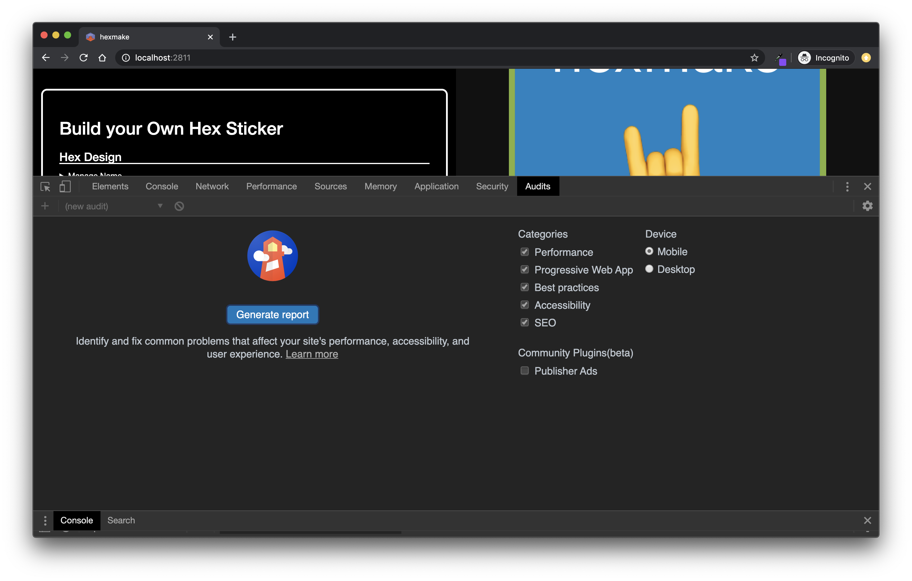
FIGURE 14.5: Launching Lighthouse audit from Google Chrome.

See Figure 14.6 for a screenshot of the results computed by Google Lighthouse.

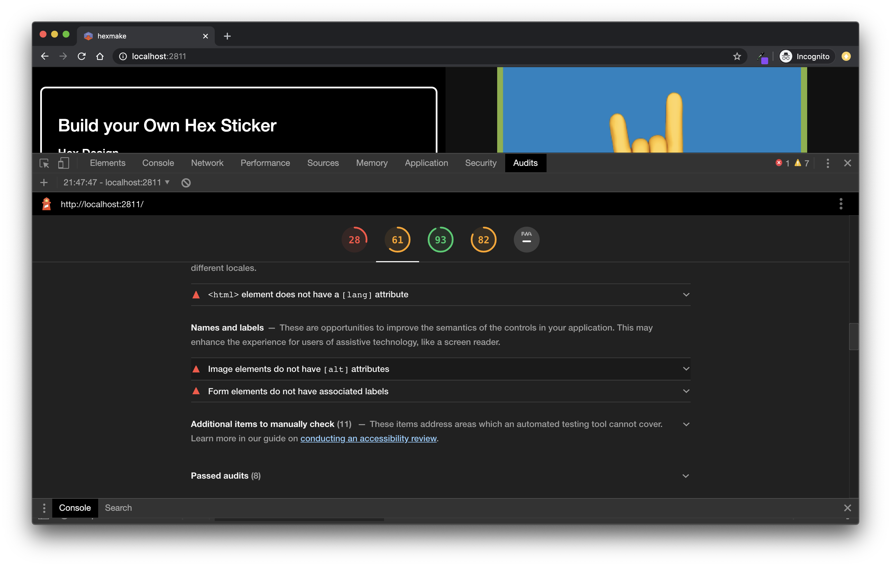
FIGURE 14.6: Lighthouse audit results.

Once the audit is finished, you have some basic but useful indications about your application:

Performance. This metric mostly analyzes the rendering time of the page: for example, how much time does it take to load the app in full, that is to say how much time it takes from the first byte received to the app being fully ready to be used, the time between the very first call to the server and the very first response, etc. With shiny (Chang et al. 2022), you should get low performance here, notably due to the fact that it is serving external dependencies that you might not be able to control. For example, the report from hexmake (Fay 2023g) suggests to “Eliminate render-blocking resources”, and most of them are not controlled by the shiny developer: they come bundled with shiny::fluidPage() itself.
Accessibility. Google Lighthouse performs a series of accessibility tests (see our chapter about accessibility for more information).
Best practices bundles a list of “misc” best practices around web applications.
SEO, search engine optimization, or how your app will perform when it comes to search engine indexation.⁵⁸
Progressive Web App (PWA): A PWA is an app that can run on any device, “reaching anyone, anywhere, on any device with a single codebase”. Google audit your application to see if your application fits with this idea.

Profiling web page is a wide topic and a lot of things can be done to enhance the global page performance. That being said, if you have a limited time to invest in optimizing the front-end performance of the application, Google Lighthouse is a perfect tool, and can be your go-to audit tool for your application.

And if you want to do it from R, the npm lighthouse module allows you to output the audit in JSON, which can then be brought back to R!

lighthouse --output json \
  --output-path data-raw/output.json \
  http://localhost:2811

Then, being a JSON file, you can call if from R:

# Reading the JSON output of your lighthouse audit, 
# and displaying the Speed Index value
lighthouse_report <- jsonlite::read_json("data-raw/output.json")
lighthouse_report$audits$`speed-index`$displayValue

[1] "5.4 s"

The results are contained in the audits sections of this object, and each of these sub-elements contains a description field, detailing what the metric means.

Here are, for example, some of the results, focused on performance, with their respective descriptions:

“First Meaningful Paint”

# Each audit point contains a description, 
# that explains what this value stands for
lighthouse_report$audits$`first-meaningful-paint`$description

[1] "First Meaningful Paint measures when the primary"
[2] "content of a page is visible. [Learn"            
[3] "more](https://web.dev/first-meaningful-paint)."

# We can turn the results into a data frame
lighthouse_report$audits$`first-meaningful-paint` %>%
  tibble::as_tibble()  %>%
  dplyr::select(title, score, displayValue)

# A tibble: 1 × 3
  title                  score displayValue
  <chr>                  <dbl> <chr>       
1 First Meaningful Paint  0.23 5.4 s

“Speed Index”

lighthouse_report$audits$`speed-index`$description

[1] "Speed Index shows how quickly the contents of a page"
[2] "are visibly populated. [Learn"                       
[3] "more](https://web.dev/speed-index)."

lighthouse_report$audits$`speed-index` %>%
  tibble::as_tibble()  %>%
  dplyr::select(title, score, displayValue)

# A tibble: 1 × 3
  title       score displayValue
  <chr>       <dbl> <chr>       
1 Speed Index  0.56 5.4 s

“Estimated Input Latency”

lighthouse_report$audits$`estimated-input-latency`$description

[1] "Estimated Input Latency is an estimate of how long"   
[2] "your app takes to respond to user input, in"          
[3] "milliseconds, during the busiest 5s window of page"   
[4] "load. If your latency is higher than 50 ms, users may"
[5] "perceive your app as laggy. [Learn"                   
[6] "more](https://web.dev/estimated-input-latency)."

lighthouse_report$audits$`estimated-input-latency` %>%
  tibble::as_tibble()  %>%
  dplyr::select(title, score, displayValue)

# A tibble: 1 × 3
  title                   score displayValue
  <chr>                   <int> <chr>       
1 Estimated Input Latency     1 10 ms

“Total Blocking Time”

lighthouse_report$audits$`total-blocking-time`$description

[1] "Sum of all time periods between FCP and Time to"       
[2] "Interactive, when task length exceeded 50ms, expressed"
[3] "in milliseconds."

lighthouse_report$audits$`total-blocking-time` %>%
  tibble::as_tibble()  %>%
  dplyr::select(title, score, displayValue)

# A tibble: 1 × 3
  title               score displayValue
  <chr>               <int> <chr>       
1 Total Blocking Time     1 30 ms

“Time to first Byte”

lighthouse_report$audits$`time-to-first-byte`$description

[1] "Time To First Byte identifies the time at which your"
[2] "server sends a response. [Learn"                     
[3] "more](https://web.dev/time-to-first-byte)."

lighthouse_report$audits$`time-to-first-byte` %>%
  .[c("title", "score", "displayValue")] %>%
  tibble::as_tibble()

# A tibble: 1 × 3
  title                              score displayValue
  <chr>                              <int> <chr>       
1 Server response times are low (TT…     1 Root docume…

Google Lighthouse also comes with a continuous integration tool, so that you can use it as a regression testing tool for your application. To know more, feel free to read the documentation!

Side note on minification

Chances are that right now you are not using minification in your shiny application. Minification is the process of removing unnecessary characters from files, without changing the way the code works, to make the file size smaller. The general idea being that line breaks, spaces, and a specific set of characters are used inside scripts for human readability, and are not useful when it comes to the way a computer reads a piece of code. Why not remove them when they are served in a larger software? This is what minification does.

Here is an example of how minification works, taken from Empirical Study on Effects of Script Minification and HTTP Compression for Traffic Reduction (Sakamoto et al. 2015):

var sum = 0;
for ( var i = 0; i <=10; i ++ ) {
  sum += i ;
}
alert( sum ) ;

is minified into:

var sum=0;for(var i=0;i<=10;i++){sum+=i};alert(sum);

Both these code blocks behave the same way, but the second one will be smaller when saved to a file: this is the very core principle of minification of files. It is something pretty common to do when building web applications: on the web, every byte counts, so the smaller your external resources the better. Minification is important as the larger your resources, the longer your application will take to launch, and:

Page launch time is crucial when it comes to ranking the pages on the web.
The larger the resources, the longer it will take to launch the application on a mobile, notably if users are visiting your application from a 3G/4G network.

And do not forget the following:

Extremely high-speed network infrastructures are becoming more and more popular in developed countries. However, we still face crowded and low-speed Wi-Fi environments on airport, cafe, international conference, etc. Especially, a network environment of mobile devices requires efficient usage of network bandwidth.

Empirical study on effects of script minification and HTTP compression for traffic reduction (Sakamoto et al. 2015)

To minify JavaScript, HTML and CSS files from R, you can use the {minifyr} (Fay 2023h) package, which wraps the node-minify NodeJS library. For example, compare the size of this file from shiny:

# Displaying the file size of a CSS file from {shiny}
fs::file_size(
  system.file("www/shared/shiny.js", package = "shiny")
)

239K

To its minified version:

# Using the {minifyr} package to minify the CSS file
minified <- minifyr::minifyr_js_gcc(
  system.file("www/shared/shiny.js", package = "shiny"), 
  "shinymini.js"
)

# Minifying can help you gain kilobytes
fs::file_size(minified)

87.5K

That might not seem like much (a couple of KB) on a small scale, but as it can be done automatically, why not leverage these small performance gains when building larger applications? Of course, minification will not suddenly make your application blazing fast, but that’s something you should consider when deploying an application to production, notably if you use a lot of packages with interactive widgets: they might contain CSS and JavaScript files that are not minified.

Minification can be important notably if you expect your audience to be connecting to your app with a low bandwidth: whenever your application starts, the browser has to download the source files from the server, meaning that the larger these files, the longer it will take to render.

Note that shiny files are minified by default, so you will not have to re-minify them. But most packages that extend shiny are not, so minifying the CSS and JavaScript files from these packages might help you win some points on you Google Lighthouse report!

To do this automatically, you can add the {minifyr} commands to your deployment, be it on your CD/CI platform, or as a Dockerfile step. {minifyr} comes with a series of functions to do that:

minify_folder_css(), minify_folder_js(), minify_folder_html() and minify_folder_json() do a bulk minification of the files found in a folder that matches the extension.
minify_package_js(), minify_package_css(), minify_package_html() and minify_package_json() will minify the CSS and JavaScript files contained inside a package installed on the machine.

Here is what it can look like inside a Dockerfile (Note that you will need to install NodeJS inside the container):

FROM rocker/shiny-verse:3.6.3

RUN apt-get -y install curl 
RUN curl -sL \
  <https://deb.nodesource.com/setup_14.x> \
  | bash - 
RUN apt-get install -y nodejs

RUN Rscript -e 'remotes::install_github("colinfay/minifyr")' 
RUN Rscript -e 'remotes::install_cran("cicerone")' 
RUN Rscript -e 'library(minifyr);\
    minifyr_npm_install(TRUE);\
    minify_package_js("cicerone", minifyr_js_uglify)'

14.2.3 More resources about web-page performance

13 Deploy Your Application

15 Common Application Caveats