3 Structuring Your Project
3.1 {shiny} app as a package
In the next chapter you will be introduced to the golem (Fay, Guyader, Rochette, et al. 2023) package, an opinionated framework for building production-ready shiny applications. This framework will be used a lot throughout this book, and it relies on the idea that every shiny application should be built as an R package.
But in a world where shiny applications are mostly created as a series of files, why bother with a package?
3.1.1 What is in a production-grade {shiny} app?
You probably haven’t realized it yet, but if you have built a significant (in terms of size or complexity of the codebase) shiny application, chances are you have been using a package-like structure without knowing it.
Think about your last shiny application, which was created as a single-file (app.R) or two-file app (ui.R and server.R).
On top of these files, what did you need to make it a production-ready application, and why is a package the perfect infrastructure?
A. It has metadata
First of all, metadata. In other words, all the necessary information for something that runs in production: the name of the app, the version number (which is crucial to any serious, production-level project), what the application does, who to contact if something goes wrong, etc.
This is what you will get when using a package DESCRIPTION file.
B. It handles dependencies
Second, you need to find a way to handle the dependencies. When you want to push your app into production, you do not want to have this conversation with the IT team:
IT: Hey, I tried to
source("app.R")as you said, but I got an error.R-dev: What is the error?
IT: It says “could not find package ‘shiny’”.
R-dev: Ah yes, you need to install {shiny}. Try to run
install.packages("shiny").IT: OK nice. What else?
R-dev: Let me think, try also
install.packages("DT")… good? Now tryinstall.packages("ggplot2"), and …[…]
IT: Ok, now I source the ‘app.R’, right?
R-dev: Sure!
IT: Ok so it says “could not find function
runApp()”R-dev: Ah, you got to do
library(shiny)at the beginning of your script. Andlibrary(purrr), andlibrary(jsonlite), and…
For example here, the library(purrr) and library(jsonlite) will lead to a NAMESPACE conflict on the flatten() function that can cause you some debugging headaches (trust us, we have been there before).
It would be cool if we could have a shiny app that only imports specific functions from a package, right?
We cannot stress enough that dependencies matter.
You need to handle them, and handle them correctly if you want to ensure a smooth deployment to production.
This dependency management is native when you use a package structure: the packages your application depends on are listed in the DESCRIPTION, and the functions/packages you need to import are listed in the NAMESPACE file.
C. It’s split into functions
Third, let’s say you are building a big application. Something with thousands of lines of code. You cannot build this large application by writing one or two files, as it is simply impossible to maintain in the long run or use on a daily basis. If we are developing a large application, we should split everything into smaller files. And maybe we can store those files in a specific directory.
This is what is done with a package, with the R/ folder.
D. It has documentation
Last but not least, we want our app to live long and prosper, which means we need to document it.
Documenting your shiny app involves explaining features to the end users and also to the future developers (chances are this future developer will be you). The good news is that using the R package structure helps you leverage the common tools for documentation in R:
A
READMEfile that you will put at the root of your package, which will document how to install the package, and some information about how to use the package. Note that in many cases developers go for a.mdfile (short for markdown) because this format is automatically rendered on services like GitHub, GitLab, or any other main version control system.Vignettesare longer-form documentation that explains in more depth how to use your app. They are also useful if you need to detail the core functions of the application using a static document, notably for prototyping and/or for exchanging with the client. We will get back toVignettesin Chapter 9 when we will talk about prototyping.Function documentation. Every function in your package should come with its own documentation, even if it is just for your future self. “Exported” functions, the ones which are available once you run
library(myapp), should be fully documented and will be listed in the package help page. Internal functions need less documentation, but documenting them is the best way to be sure you can come back to the app in a few months and still know why things are the way they are, what the pieces of the apps are used for, and how to use these functions.18If needed, you can build a pkgdown website, that can either be deployed on the web or kept internally. It can contain installation steps for I.T., internal features use for developers, a user guide, etc.
E. It’s tested
The other thing we need for our application to be successful in the long run is a testing infrastructure, so that we are sure we are not introducing any regression during development.
Nothing should go to production without being tested. Nothing.
Testing production apps is a broad question that we will come back to in another chapter, but let’s talk briefly about why using a package structure helps with testing.
Frameworks for package testing are robust and widely documented in the R world, and if you choose to embrace the “shiny app as a package” structure, you do not have to put in any extra-effort for testing your application back-end: use a canonical testing framework like testthat (Wickham 2023a). Learning how to use it is not the subject of this chapter, so feel free to refer to the documentation, and see also Chapter 5 of the workshop: “Building a Package that Lasts”.
We will come back to testing in Chapter 11: “Build Yourself a Safety Net”.
F. There is a native way to build and deploy it
Oh, and it would also be nice if people could get a tar.gz and install it on their computer and have access to a local copy of the app!
Or if we could install that on the server without any headache!
When adopting the package structure, you can use classical tools to locally install your shiny application, i.e. as any other R package, built as a tar.gz.
On a server, be it RStudio products or as Docker containers, the package infrastructure will also allow you to leverage the native R tools to build, install and launch R code.
More about this in Chapter 13.
3.2 Using {shiny} modules
Modules are one of the most powerful tools for building shiny applications in a maintainable and sustainable manner.
3.2.1 Why {shiny} modules?
Small is beautiful.
Being able to properly cut a codebase into small modules will help developers build a mental model of the application (Remember “What is a complex {shiny} application?”).
But what are shiny modules?
shiny modules address the namespacing problem in shiny UI (User Interface) and server logic, adding a level of abstraction beyond functions.
Modularizing Shiny app code (https://shiny.rstudio.com/articles/modules.html)
Let us first untangle this quote with an example about the shiny namespace problem.
B. Working with a bite-sized codebase
Build your application through multiple smaller applications that are easier to understand, develop and maintain, using shiny (Chang et al. 2022) modules.
We assume that you know the saying that “if you copy and paste something more than twice, you should make a function”. In a shiny application, how can we refactor a partially repetitive piece of code so that it is reusable?
Yes, you guessed right: using shiny modules. shiny modules aim at three things: simplify “id” namespacing, split the codebase into a series of functions, and allow UI/Server parts of your app to be reused. Most of the time, modules are used to do the two first. In our case, we could say that 90% of the modules we write are never reused;19 they are here to allow us to split the codebase into smaller, more manageable pieces.
With shiny modules, you will be writing a combination of UI and server functions. Think of them as small, standalone shiny apps, which handle a fraction of your global application. If you develop R packages, chances are you have split your functions into series of smaller functions. With shiny modules, you are doing the exact same thing: with just a little bit of tweaking, you can split your application into a series of smaller applications.
3.2.2 When to use {shiny} modules
No matter how big your application is, it is always safe to start modularizing from the very beginning. The sooner you use modules, the easier downstream development will be. It is even easier if you are working with golem, which promotes the use of modules from the very beginning of your application.
“Yes, but I just want to write a small app, nothing fancy.”
A production app almost always started as a small proof of concept. Then, the small PoC becomes an interesting idea. Then, this idea becomes a strategic asset. And before you know it, your not-that-fancy app needs to become larger and larger. So, you will be better off starting on solid foundations from the very beginning.
3.2.3 A practical walkthrough
An example is worth a thousand words, so let’s explore the code of a very small shiny application that is split into modules.
A. Your first {shiny} module
Let’s try to transform the above example (the one with two sliders and two action buttons) into an application with a module. Note that the following code will work only for shiny version 1.5.0 and after.
# Re-usable module
choice_ui <- function(id) {
  # This ns <- NS structure creates a
  # "namespacing" function, that will
  # prefix all ids with a string
  ns <- NS(id)
  tagList(
    sliderInput(
      # This looks the same as your usual piece of code,
      # except that the id is wrapped into
      # the ns() function we defined before
      inputId = ns("choice"),
      label = "Choice",
      min = 1, max = 10, value = 5
    ),
    actionButton(
      # We need to ns() all ids
      inputId = ns("validate"),
      label = "Validate Choice"
    )
  )
}

choice_server <- function(id) {
  # Calling the moduleServer function
  moduleServer(
    # Setting the id
    id,
    # Defining the module core mechanism
    function(input, output, session) {
      # This part is the same as the code you would put
      # inside a standard server
      observeEvent( input$validate , {
        print(input$choice)
      })
    }
  )
}


# Main application
library(shiny)
app_ui <- function() {
  fluidPage(
    # Call the UI  function, this is the only place
    # your ids will need to be unique
    choice_ui(id = "choice_ui1"),
    choice_ui(id = "choice_ui2")
  )
}

app_server <- function(input, output, session) {
  # We are now calling the module server functions
  # on a given id that matches the one from the UI
  choice_server(id = "choice_ui1")
  choice_server(id = "choice_ui2")
}

shinyApp(app_ui, app_server)
Let’s stop for a minute and decompose what we have here.
The server function of the module (mod_server()) is pretty much the same as before: you use the same code as the one you would use in any server part of a shiny application.
The ui function of the module (mod_ui()) requires specific things.
There are two new things: ns <- NS(id) and ns(inputId).
That is where the namespacing happens.
Remember the previous version where we identified our two “validate” buttons with slightly different namespaces: validate1 and validate2?
Here, we create namespaces with the ns() function, built with ns <- NS(id).
This line, ns <- NS(id), is added on top of all module UI functions and will allow building namespaces with the module id.
To understand what it does, let us try and run it outside shiny:
# Defining the id
id <- "mod_ui_1"
# Creating the internal "namespacing" function
ns <- NS(id)
# "namespace" the id
ns("choice")
[1] "mod_ui_1-choice"And here it is, our namespaced id!
Each call to a module with choice_server() requires a different id argument that will allow creating various internal namespaces to prevent from id conflicts.20
Then you can have as many validate ids as you want in your whole app, as long as this input has a unique id inside your module.
Note for {shiny} < 1.5.0
Released on 2020-06-23, the version 1.5.0 of shiny introduced a new way to write shiny modules, using a new function called moduleServer().
This new function was introduced to make the couple ui_function / server_function more obvious, where the old version used to require a callModule(server_function, id) call.
This callModule notation is still valid (at least at the time of writing these lines), but we chose to go for the moduleServer() notation in this book.
Most of the applications that are used as examples in this book have been built before this new function though, so when you will read their code, you will find the callModule implementation.
B. Passing arguments to your modules
shiny modules will potentially be reused and may need a specific user interface and inputs. This requires using extra arguments to generate the UI and server. As the UI and server are functions, you can set parameters that will be used to configure the internals of the result.
As you can see, the app_ui contains a series of calls to the
mod_ui(unique_id, ...) function, allowing additional arguments like any other function:
mod_ui <- function(id, button_label) {
  ns <- NS(id)
  tagList(
    actionButton(ns("validate"), button_label)
  )
}

# Printing the HTML for this piece of UI
mod_ui("mod_ui_1", button_label = "Validate ")
mod_ui("mod_ui_2", button_label = "Validate, again")
<!-- The ids are "namespaced" with mod_ui_*-->
<button id="mod_ui_1-validate" type="button"
class="btn btn-default action-button">Validate</button>
<!-- The ids are "namespaced" with mod_ui_*-->
<button id="mod_ui_2-validate" type="button"
class="btn btn-default action-button">Validate, again</button>The app_server side contains a series of mod_server(unique_id, ...), also allowing additional parameters, just like any other function.
As a live example, we can have a look at mod_dataviz.R from the tidytuesday201942 (Fay 2023l) shiny application, available at https://connect.thinkr.fr/tidytuesday201942/. Figure 3.1 is a screenshot of this application.
This application contains 6 tabs, 4 of them being pretty much alike: a side bar with inputs, a main panel with a button, and the plot. This plot can be, depending on the tab, a scatterplot, a histogram, a boxplot, or a barplot.
This is a typical case where you should reuse modules: if several parts are relatively similar, it is easier to bundle it inside a reusable module, and condition the UI/server with function arguments.
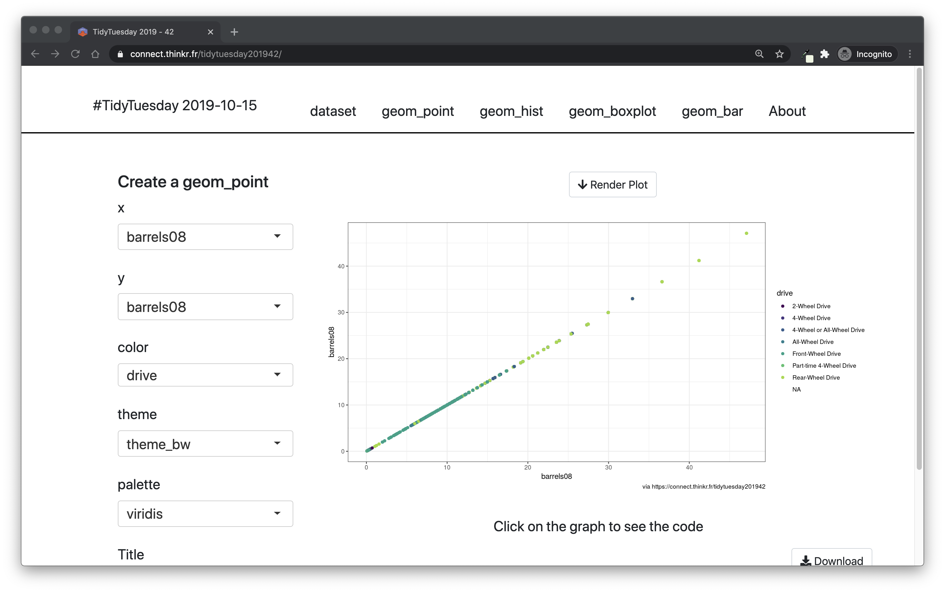
FIGURE 3.1: Snapshot of the tidytuesday201942 shiny application.
Let’s extract some pieces of this application to show how (and why) you would parametrize your module.
mod_dataviz_ui <- function(
  id,
  type = c("point", "hist", "boxplot", "bar")
) {
  # Setting a header with the specified type of graph
  h4(
    sprintf( "Create a geom_%s", type )
  ),
  # [ ... ]
  # We want to allow a coord_flip only with barplots
  if (type == "bar"){
    checkboxInput(
      ns("coord_flip"),
      "coord_flip"
    )
  },
  # [ ... ]
  # We want to display the bins input only
  # when the type is histogram
  if (type == "hist") {
    numericInput(
      ns("bins"),
      "bins",
      30,
      1,
      150,
      1
    )
  },
  # [ ... ]
  # The title input will be added to the graph
  # for every type of graph
  textInput(
    ns("title"),
    "Title",
    value = ""
  )
}
And in the module server:
mod_dataviz_server <- function(
  input,
  output,
  session,
  type
) {
  # [ ... ]
  if (type == "point") {
    # Defining the server logic when the type is point
    # When the type is point, we have access to input$x,
    # input$y, input$color, and input$palette,
    # so we reuse them here
    ggplot(
      big_epa_cars,
      aes(
        .data[[input$x]],
        .data[[input$y]],
        color = .data[[input$color]])
    )  +
      geom_point()+
      scale_color_manual(
        values = color_values(
          1:length(
            unique(
              pull(
                big_epa_cars,
                .data[[input$color]])
            )
          ),
          palette = input$palette
        )
      )
  }
  # [ ... ]
  if (type == "hist") {
    # Defining the server logic when the type is hist
    # When the type is point, we have access to input$x,
    # input$color, input$bins, and input$palette
    # so we reuse them here
    ggplot(
      big_epa_cars,
      aes(
        .data[[input$x]],
        fill = .data[[input$color]]
      )
    ) +
      geom_histogram(bins = input$bins)+
      scale_fill_manual(
        values = color_values(
          1:length(
            unique(
              pull(
                big_epa_cars,
                .data[[input$color]]
              )
            )
          ),
          palette = input$palette
        )
      )
  }
}
Then, the UI of the entire application is:
app_ui <- function() {
  # [...]
  tagList(
    fluidRow(
      # Setting the first tab to be of type point
      id = "geom_point",
      mod_dataviz_ui(
        "dataviz_ui_1",
        type = "point"
      )
    ),
    fluidRow(
      # Setting the second tab to be of type point
      id = "geom_hist",
      mod_dataviz_ui(
        "dataviz_ui_2",
        type = "hist"
      )
    )
  )
}
And the app_server() of the application:
app_server <- function(input, output, session) {
  # This app has been built before shiny 1.5.0,
  # so we use the callModule structure
  #
  # We here call the server module on their
  # corresponding id in the UI, and set the
  # parameter of the server function to
  # match the correct type of input
  callModule(mod_dataviz_server, "dataviz_ui_1", type = "point")
  callModule(mod_dataviz_server, "dataviz_ui_2", type = "hist")
}
3.2.4 Communication between modules
One of the hardest part of using modules is sharing data across them. There are at least three approaches:
- Returning a
reactivefunction - The “stratégie du petit r” (to be pronounced with a French accent of course)
- The “stratégie du grand R6”
A. Returning values from the module
One common approach is to return a reactive function from one module, and pass it to another in the general app_server() function.
Here is an example that illustrates this pattern.
# Module 1, which will allow to select a number
choice_ui <- function(id) {
  ns <- NS(id)
  tagList(
    # Add a slider to select a number
    sliderInput(ns("choice"), "Choice", 1, 10, 5)
  )
}


choice_server <- function(id) {
  moduleServer( id, function(input, output, session) {
    # We return a reactive function from this server,
    # that can be passed along to other modules
    return(
      reactive({
        input$choice
      })
    )
  }
  )
}

# Module 2, which will display the number
printing_ui <- function(id) {
  ns <- NS(id)
  tagList(
    # Insert the number modified in the first module
    verbatimTextOutput(ns("print"))
  )
}

printing_server <- function(id, number) {
  moduleServer(id, function(input, output, session) {
    # We evaluate the reactive function
    # returned from the other module
    output$print <- renderPrint({
      number()
    })
  }
  )
}

# Application
library(shiny)
app_ui <- function() {
  fluidPage(
    choice_ui("choice_ui_1"),
    printing_ui("printing_ui_2")
  )
}

app_server <- function(input, output, session) {
  # choice_server() returns a value that is then passed to
  # printing_server()
  number_from_first_mod <- choice_server("choice_ui_1")
  printing_server(
    "printing_ui_2",
    number = number_from_first_mod
  )
}

shinyApp(app_ui, app_server)
This strategy works well, but for large shiny apps it might be hard to handle large lists of reactive outputs / inputs and to keep track of how things are organized.
It might also create some reactivity issues, as a lot of reactive function calls is harder to control, or lead to too much computation from the server.
B. The “stratégie du petit r”
In this strategy, we create a global reactiveValues list that is passed along through other modules.
The idea is that it allows you to be less preoccupied about what your module takes as input and what it outputs.
You can think of this approach as creating a small, internal database that is passed along through all the modules of your application.
Below, we create a “global” (in the sense that it is initiated at the top of the module hierarchy) reactiveValues() object in the app_server() function.
It will then go through all modules, passed as a function argument.
# Module 1, which will allow to select a number
choice_ui <- function(id) {
  ns <- NS(id)
  tagList(
    # Add a slider to select a number
    sliderInput(ns("choice"), "Choice", 1, 10, 5)
  )
}

choice_server <- function(id, r) {
  moduleServer(
    id,
    function(input, output, session) {
      # Whenever the choice changes, the value inside r is set
      observeEvent( input$choice , {
        r$number_from_first_mod <- input$choice
      })

    }
  )
}

# Module 2, which will display the number
printing_ui <- function(id) {
  ns <- NS(id)
  tagList(
    # Insert the number modified in the first module
    verbatimTextOutput(ns("print"))
  )
}

printing_server <- function(id, r) {
  moduleServer(
    id,
    function(input, output, session) {
      # We evaluate the reactiveValue element modified in the
      # first module
      output$print <- renderPrint({
        r$number_from_first_mod
      })
    }
  )
}

# Application
library(shiny)
app_ui <- function() {
  fluidPage(
    choice_ui("choice_ui_1"),
    printing_ui("printing_ui_2")
  )
}

app_server <- function(input, output, session) {
  # both servers take a reactiveValue,
  #  which is set in the first module
  # and printed in the second one.
  # The server functions don't return any value per se
  r <- reactiveValues()
  choice_server("choice_ui_1", r = r)
  printing_server("printing_ui_2", r = r)
}

shinyApp(app_ui, app_server)
The good thing about this method is that whenever you add something in one module, it is immediately available in all other modules where r is present.
The downside is that it can make it harder to reason about the app, as the input/content of the r is not specified anywhere unless you explicitly document it: the parameter to your server function being “r” only, you need to be a little bit more zealous when it comes to documenting it.
Note that if you want to share your module, for example in a package, you should document the structure of the r.
For example:
#' @param r a `reactiveValues()` list with a
    `number_from_first_mod` element in it.
#' This `r$number_from_first_mod` will be
    printed to the `print` output.
C. The “stratégie du grand R6”
Similar to the “stratégie du petit r”, we can create an R6 object, which is passed along inside the modules.
R6 objects, created using the package of the same name, are “traditional” object-oriented programming implementations in R. An R6 object is a data structure that can hold in itself data and functions. Its particularity is that if it’s modified inside a function, this modified value is kept outside the function in which it’s called, making it a powerful tool to manage data across the application.
As this R6 object is not a reactive object and is not meant to be used as such, uncontrolled reactivity of the application is reduced, thus reduces the complexity of handling chain reactions across modules.
Of course, you need to have another special tool in your app to trigger elements.
All this will be explained in detail in Chapter 15 of this book, and you can find an example of this pattern inside the {hexmake} (Fay 2023g) application.
If you are eager to know more about what R6 is and how it works, we suggest the chapter on this subject in Advanced R (Wickham 2019), R6.
D. Other approaches: About {tidymodules}
tidymodules (Larbaoui 2023) is a package that helps in building shiny modules using an object-oriented paradigm, based on R6. It allows you to automatically take care of namespaces, and makes sharing data across modules easier. With this approach, as modules are objects, you can also define inheritance between modules.
The “Getting Started” page for tidymodules offers a presentation of how you can build modules using this approach, so feel free to refer to it if you want to know more, and to dive into the article for the advanced features offered by this package.
3.3 Structuring your app
3.3.1 Business logic and application logic
A shiny application has two main components: the application logic and the business logic.
Application logic is what makes your shiny app interactive: structure, buttons, tables, interactivity, etc. These components are not specific to your core business. You could use them for any other line of work or professional context. This has no other use case than your interactive application. It is not meant to be used outside your app, and you would not use them in a markdown report for instance.
Business logic includes the components with the core algorithms and functions that make your application specific to your area of work. You can recognize these elements as the ones that can be run outside any interactive context. This is the case for specific computations and algorithms, custom plots or
geomfor ggplot2 (Wickham, Chang, et al. 2023), specific calls to a database, etc.
These two components do not have to live together.
And in reality, they should not live together if you want to keep your sanity when you are building an app.
If you keep all components together in the same file, you will end up having to rerun the app from scratch and spend five minutes clicking everywhere just to be sure you have correctly set the color palette for the graph on the last tabPanel().
Trust us, we have been there, and it is not pretty.
What is the way to go? Extract the business function from the reactive functions. Literally. Compare this pattern:
library(shiny)
library(dplyr)
# A simple app that returns a table
ui <- function() {
  tagList(
    tableOutput("tbl"),
    sliderInput("n", "Number of rows", 1, 50, 25)
  )
}

server <- function(input, output, session) {
  output$tbl <- renderTable({
    # Writing all the business logic for the table manipulation
    # inside the server
    mtcars %>%
      # [...] %>%
      # [...] %>%
      # [...] %>%
      # [...] %>%
      # [...] %>%
      top_n(input$n)
  })
}

shinyApp(ui, server)
To this one:
library(shiny)
library(dplyr)

# Writing all the business logic for the table manipulation
# inside an external function
top_this <- function(tbl, n) {
  tbl %>%
    # [...] %>%
    # [...] %>%
    # [...] %>%
    # [...] %>%
    top_n(n)
}

# A simple app that returns a table
ui <- function() {
  tagList(
    tableOutput("tbl"),
    sliderInput("n", "Number of rows", 1, 50, 25)
  )
}


server <- function(input, output, session) {
  output$tbl <- renderTable({
    # We call the previously declared function inside the server
    # The business logic is thus defined outside the application
    top_this(mtcars, input$n)
  })
}

shinyApp(ui, server)
Both scripts do the exact same thing.
The difference is that the second code can be easily explored without having to relaunch the app.
You will be able to build a reproducible example to explore, illustrate, and improve top_this().
This function can be tested, documented, and reused outside the application.
Moreover, this approach lowers the cognitive load when debugging: you either debug an application issue, or a business logic issue.
You never debug both at the same time.
Even more, think about the future: how likely are the colors or the UI subject to change, compared to how likely the core algorithms are to change? As said in The Art of Unix Programming, “Fashions in the look and feel of GUI toolkits may come and go, but raster operations and compositing are forever” (Raymond 2003). In other words, the core back-end, once consolidated, will potentially stay unchanged forever. On the other hand, the front-end might change: new colors, new graphic designs, new interactions, new visualization libraries, etc. Whenever this happens, you will be happy you have separated the business logic from the application logic, as you will have to change less code.
How to do that?
Add your application logic in a file (typically, a module), and the business logic in another R script (typically starting with fct_ or utils_).
You can even write the business logic inside another package, making these functions really reusable outside your application.
3.3.2 Small is beautiful (bis repetita)
There are a lot of reasons for splitting your application into smaller pieces, including the fact that it is easier to maintain, easier to decipher, and it facilitates collaboration.
There is nothing harder to maintain than a shiny app only made of a unique 1000-line long app.R file.
Well, there still is the 10000-line long app.R file, but you get the idea.
Long scripts are almost always synonymous with complexity when it comes to building software.
Of course, small and numerous scripts do not systematically prevent codebase complexity, but they do simplify collaboration and maintenance, and divide the application logic into smaller, easier-to-understand bits of code.
In practice, big files are complex to handle and make development harder. Here is what happens when you work on an application for production:
You will work during a long period of time (either in one run or split across several months) on your codebase. Hence, you will have to get back to pieces of code you wrote a long time ago.
You will possibly develop with other developers. Maintaining a codebase when several people work on the same directory is already a complex thing: from time to time you might work on the same file separately, a situation where you will have to be careful about what and how to merge things when changes are implemented. It is almost impossible to work together on the same file throughout the project without losing your mind: even more if this file is thousands of lines long.
You will implement numerous features. Numerous features imply a lot of UI and server interactions. In an
app.Rfile containing thousands of lines, it is very hard to match the UI element with its server counterpart. When the UI is on line 50 and the server on line 570, you will be scrolling a lot when working on these elements.
3.3.3 Conventions matter
In this section you will find a suggestion for a naming convention for your app files that will help you and your team be organized.
Splitting files is good. Splitting files using a defined convention is better. Why? Because using a common convention for your files helps the other developers (and potentially you) to know exactly what is contained in a specific file, making it easier to navigate through the codebase, be it for newcomers or for developers already familiar with the software.
As developed in Refactoring at Scale (Lemaire 2020), lacking a defined file structure when it comes to the codebase leads to slower productivity in the long run, notably when new engineers join the team: engineers with a knowledge of the file structure have learned how to navigate through the codebase, but new comers will find it hard to understand how everything is organized. And of course, in the long run, even developers with a knowledge of the structure can get lost, even more if they haven’t worked on the project for months.
Because it’s easier to maintain the status quo, instead of proactively beginning to organize related files […], engineers instead learn to navigate the increasingly sprawling code. New engineers introduced to the growing chaos raise a warning flag and encourage the team to begin splitting up the code, but these concerns fall to deaf ears […]. Eventually, the codebase reaches a critical mass where the persistent lack of organization has dramatically slowed productivity across the engineering team. Only then does the team take the time to draft a plan for grooming the codebase, at which point the number of variables to consider is far greater than had they made a concerted effort to tackle the problem months (or even years) earlier.
Refactoring at Scale (Lemaire 2020)
Using a convention allows everyone to know where to look when debugging, refactoring, or implementing new features.
For example, if you follow golem’s convention (which is the one developed in this section), you will know immediately that a file starting with mod_ contains a module.
If you take over a project, look in the R/ folder, and see files starting with these three letters, you will know immediately that these files contain modules.
Here is our proposition for a convention defining how to split your application into smaller pieces.
First of all, put everything into an R/ folder.
If you build your app using the golem framework, this is already the case.
We use the package convention to hold the functions of our application.
The naming convention in golem is the following:
app_*.R(typicallyapp_ui.Randapp_server.R) contain the top-level functions defining your user interface and your server function.fct_*files contain the business logic, which are potentially large functions. They are the backbone of the application and may not be specific to a given module. They can be added using golem with theadd_fct("name")function.mod_*files contain a unique module. Many shiny apps contain a series of tabs, or at least a tab-like pattern, so we suggest that you number them according to their step in the application. Tabs are almost always named in the user interface, so that you can use this tab name as the file name. For example, if you build a dashboard where the first tab is called “Import”, you should name your filemod_01_import.R. You can create this file with a module skeleton usinggolem::add_module("01_import").utils_*are files that contain utilities, which are small helper functions. For example, you might want to have anot_na, which isnot_na <- Negate(is.na), anot_null, or small tools that you will be using application-wide. Note that you can also createutilsfor a specific module.*_ui_*, for exampleutils_ui.R, relates to the user interface.*_server_*are files that contain anything related to the application’s back-end. For example,fct_connection_server.Rwill contain functions that are related to the connection to a database, and are specifically used from the server side.
Note that when building a module file with golem, you can also create fct_ and utils_ files that will hold functions and utilities for this specific module.
For example, golem::add_module("01_import", fct = "readr", utils = "ui") will create R/mod_01_import.R, R/mod_01_import_fct_readr.R and R/mod_01_import_utils_ui.R.
Of course, as with any convention, you might occasionally feel like deviating from the general pattern.
Your app may not have that many functions, or maybe the functions can all fit into one utils_ file.
But whether you have one or thousands of files, it is always a good practice to stick to a formalized pattern as much as possible.