1 About Successful {shiny} Apps
1.1 A (very) short introduction to {shiny}
If you are reading this page, chances are you already know what a shiny application (sometimes shortened as “shiny app”) is—a web application that communicates with R, built in R, and working with R. The beauty of shiny (Chang et al. 2022) is that it makes it easy for someone already familiar with R to create a small app in a matter of hours. With small and minimal shiny apps, no knowledge of HTML (HyperText Markup Language), CSS(Cascading Style Sheets) or JavaScript is required, and you do not have to think about technical elements that usually come with web applications—for example, you do not have to think about the port the application is served on: shiny picks one for you.4 Same goes for serving external dependencies: the application comes with its set of CSS and JavaScript dependencies that a common shiny developer does not need to worry about. And that is probably one of the main reasons why this package has become so successful over the years—with very little training, you can rapidly create a proof-of-concept (PoC) for a data product, showcase an algorithm, or present your results in an elegant and accessible user interfaces.
The first version of shiny was published in 2012.
Since then, it has been one of the top projects of the RStudio team.
At the time of writing these lines (April 2020), there are more than 4700 commits in the master branch of the GitHub repository, made by 46 contributors.
It is now downloaded around 400K times a month, according to cranlogs, and has 1174 reverse dependencies (i.e. packages that depend on it), according to revdep("shiny") from devtools (Wickham, Hester, et al. 2022).
If you are very new to shiny, this book might feel a little bit overwhelming: we will be discussing some advanced shiny and software engineering methods, best practices and structural ideas for sending shiny applications to production. This book relies on the assumption that you already know how to build basic shiny applications, and that you want to push your shiny skills to the next level: in other words, you are ready to move from the Proof of Concept to the production-grade application. If you are very new to shiny, we suggest you start with the Mastering Shiny book before reading the present book.
Ready to start engineering production-grade shiny apps?
1.2 What is a complex {shiny} application?
One of the unfortunate things about reality is that it often poses complex problems that demand complex solutions.
The Art of Unix Programming (Raymond 2003)
1.2.1 Reaching the cliff of complexity
Building a shiny application seems quite straightforward when it comes to small prototypes or proof of concepts: after a few hours of practice and documentation reading, most R developers can have a small working application.
But things change when your application reaches “the cliff of complexity”,5 i.e. that moment when the application reaches a state when it can be qualified as “complex”.
But what do we mean by complexity? Getting a clear definition is not an easy task 6 as it very much depends on who is concerned and who you are talking to. But a good definition can be found in The DevOps Handbook (Kim 2016): “One of the defining characteristics of a complex system is that it defies any single person’s ability to see the system as a whole and understand how all the pieces fit together. Complex systems typically have a high degree of interconnectedness of tightly coupled components, and system-level behavior cannot be explained merely in terms of the behavior of the system components.” (Our bold.)
Or as noted in Refactoring at Scale (Lemaire 2020), “It becomes nearly impossible to reason about the effect a change might have when applied uniformly across a sprawling, complex system. Many tools exist to identify code smells or automatically detect improvements within subsections of code, but we are largely unable to automate human reasoning about how to restructure large applications, in codebases that are growing at an increasingly rapid pace.”
Building on top of these quotes, let’s try to come up with a definition that will serve us in the context of engineering shiny applications.
When building software, we can think of complexity from two points of view: the complexity as it is seen by the developer, and the complexity as it is seen by the customer/end user.7
For the code, bugs are harder to anticipate: it is hard to think about all the different paths the software can follow and difficult to identify bugs because they are deeply nested in the numerous routines the app is doing. It is also hard to think about what the state of your app is at a given moment because of the numerous inputs and outputs your app contains.
From the user perspective, the more complex an app is, the steeper the learning curve. Indeed, the user will have to invest more time learning how the app works, and will be even more disappointed if ever they realize this time has been a waste.
Let’s dive a little bit more into these two types of complexity.
A. Developer complexity
An app is to be considered complex when it is so large in terms of size and functionality that it makes it impossible to reason about it at once, and developers must rely on tools and methods to understand and handle this complexity: for example, when it comes to shiny, you will rely on tools like the golem (Fay, Guyader, Rochette, et al. 2023) framework, introduced throughout this book, to handle some implementation, development and deployment complexity. This book will introduce a clear methodology that comes with a series of conventions, which are crucial when it comes to building and maintaining complex systems: by imposing a formalized structure for software, it enhances its readability, lowers the learning curve for newcomers, and reduces the risk of errors inherent in repetitive tasks.
This type of complexity is called implementation complexity. One of the goals of this book is to present a methodology and toolkit that will help you reduce this form of complexity.
B. Customer and user complexity
Customers and end users see complexity as interface complexity.
Interface complexity can be driven by a lot of elements, for example, the probability of making an error while using the app, the difficulty in understanding the logical progression in the app, the presence of unfamiliar behavior or terms, visual distractions, etc. This book will also bring you strategy to help you cope with the need for simplification when it comes to designing an interface.
1.2.2 Balancing complexities
There is an inherent tension between these two sources of complexity, as designing an app means finding a good balance between implementation and interface complexity. Lowering one source of complexity usually means increasing the other, and managing an application project means knowing where to draw the line. This usually requires restraining yourself from implementing too many features, and still creating an application that is easy to use, and that fits the requirements you have received.
For example, there is something common in shiny applications: what we can call the “too much reactivity pattern”. In some cases, developers try to make everything reactive: e.g., three sliders and a drop-down input, all updating a single plot. This behavior lowers the interface complexity: users do not have to really think about what they are doing, they move sliders, change the inputs, and boom! the plot updates. But this kind of pattern can make the application perform too much computation, for example, because users rarely go to the value they need on their first try: they usually miss the value they actually want to select.
One solution can be to delay reactivity or to cache things so that R computes fewer things. But that comes with a cost: handling delayed reactivity and caching elements increase implementation complexity. Another solution is to add an “update plot” button, which updates the plot only when the user clicks on it. This pattern makes it easier to control reactivity from the implementation side. But this can make the interface a little bit more complex for the users, who have to perform another action, on top of changing their inputs. We will argue in this book that not enough reactivity is better than too much reactivity, as the latter increases computation time, and relies on the assumption that the user makes the right action on the first try.
Another good example is shiny’s dateRangeInput() function.
This function requires the user to choose a start date and an end date.
However, the function allows the user to choose a start date which is after the end (that is the behavior of the JavaScript plugin used in shiny to create this input).
But allowing this behavior leads to bugs, notably in a context of full reactivity.
Handling this special case is completely doable: with a little bit of craft, you can watch what the user inputs and throw an error if the start is after the end.8
On one hand, that solution increases implementation complexity, while on the other hand, allowing this naive behavior requires the user to think carefully about what they are selecting, thus increasing the interface complexity.
What should we do? It’s up to you: deciding where to draw the line between interface and implementation complexity very much depends on the project, but that is something that you should keep in mind throughout the project’s life.
1.2.3 Assessing code complexity
On the developer side, you will want to reduce code complexity so that everybody involved in the coding process is able to create a mental model of how the application works. On the user side, you will want to reduce interface complexity so that everybody comes out of using your application with a good user experience.
Reducing complexity first comes with being able to identify its potential sources, be it in your application codebase or in the specifications describing how the application should work. Finding these sources of complexity is not an easy task, as it requires some programming knowledge to identify bottlenecks, basic UX (User Experience) skills to implement a good interface, and of course a project management methodology to structure the whole life of your application.
All these points will be addressed in this book. But before that, let’s dive into code complexity.
A. Codebase size
The total number of lines of code, and the number of files, can be good clue of potential complexity, but only if used as an order of magnitude (for example, a 10,000-line codebase is potentially more complex than a 100-line codebase), but should not be relied on if used strictly, even more if you try to reduce the number of lines by sacrificing code readability.
R is very permissive when it comes to indentation and line breaks, and, unlike JavaScript or CSS, it is generally not minified.9
In R, the number of lines of code depends on your coding style and the packages you are using. For example, the tidyverse (Wickham et al. 2019) style guide encourages the use of %>% (called “pipe”), with one function by line, producing more lines in the end code: “%>% should always have a space before it, and should usually be followed by a new line” (tidyverse style guide).
So you can expect a “tidyverse-centric” package to contain more lines of code, yet the pipe itself has been thought of as a tool to lower code complexity by enhancing its readability.10
For example, the two following pieces of code do the same thing. Both have a different number of lines, and a different level of reading complexity.
library(dplyr, warn.conflicts = FALSE)
# With pipe
iris %>%
  group_by(Species) %>%
  summarize(mean_sl = mean(Sepal.Length))
# Without the pipe
summarize(group_by(iris, Species), mean_sl = mean(Sepal.Length))
Also, there is no limit in the way you can indent your code.
# Putting one symbol by line
iris[
  1
  :
    5,
  "Species"
]
Six lines of code for something that could also be written in one line.
# Same code but everything is on the same line
iris[1:5, "Species"]
In other words, using this kind of writing style can make the codebase larger in term of lines, without really adding complexity to the general program.
Another drawback of this metric is that it focuses on numbers instead of readability, and in the long run, yes, readability matters. As noted in The Art of Unix Programming, “Pressure to keep the codebase size down by using extremely dense and complicated implementation techniques can cause a cascade of implementation complexity in the system, leading to an un-debuggable mess” (Raymond 2003).
Still, this metric can be useful to reinforce what you have learned from other metrics. It is rather unlikely that you will find this “extreme” coding style we showed above, and even if it might not make sense to compare two codebases that just differ by 1% or 2 % of lines of code, it is very likely that a codebase which is ten, one hundred, one thousand times larger is a more complex software.
Another good metric related to code complexity is the number of files in the project: R developers tend to split their functions into several files, so the more files you will find in a project, the larger the codebase is. And numerous files can also be a sign of maintenance complexity, as it may be harder to reason about an app logic that is split into several files than about something that fits into one linear code inside one file.11 On the other hand, one big 10,000-line file which is standing alone in the project is not a good sign either.
If you want to use the number-of-lines metric, you can do it from R with the cloc (Rudis and Danial 2020) package, available at https://github.com/hrbrmstr/cloc.
# Install {cloc} from GitHub
remotes::install_github("hrbrmstr/cloc")
For example, let’s compare a rather big package (shiny) with a small one (attempt (Fay 2020)):
library(cloc)
# Using dplyr to manipulate the results
library(dplyr, warn.conflicts = FALSE)

# Computing the number of lines of code
# for various CRAN packages
shiny_cloc <- cloc_cran(
  "shiny",
  .progress = FALSE,
  repos = "http://cran.irsn.fr/"
)
attempt_cloc <- cloc_cran(
  "attempt",
  .progress = FALSE,
  repos = "http://cran.irsn.fr/"
)

clocs <- bind_rows(
  shiny_cloc,
  attempt_cloc
)

# Summarizing the number of line of code inside each package
clocs %>%
  group_by(pkg) %>%
  summarise(
    loc = sum(loc)
  )
# A tibble: 2 × 2
pkg loc
<chr> <int>
1 attempt 6486
2 shiny 175376
# Summarizing the number of files inside each package
clocs %>%
  group_by(pkg) %>%
  summarise(
    files = sum(file_count)
  )
# A tibble: 2 × 2
pkg files
<chr> <int>
1 attempt 64
2 shiny 736Here, with these two metrics, we can safely assume that shiny is a more complex package than attempt.
If you want to compute the same prefix for a local package/repository, the cloc_pkg() function can be used.
For example, here is how to compute the cloc metric for the hexmake application:
# Calling the function on the {hexmake}
# application Git repository
hexmake_cloc <- cloc_git(
  "https://github.com/ColinFay/hexmake"
)
hexmake_cloc
# A tibble: 10 × 10
source language file_count file_count_pct loc
<chr> <chr> <int> <dbl> <int>
1 hexmake JSON 1 0.0102 3844
2 hexmake R 34 0.347 2345
3 hexmake Markdown 5 0.0510 95
4 hexmake CSS 1 0.0102 76
5 hexmake Dockerfile 2 0.0204 45
6 hexmake JavaScript 2 0.0204 31
7 hexmake Rmd 2 0.0204 18
8 hexmake HTML 1 0.0102 14
9 hexmake YAML 1 0.0102 8
10 hexmake SUM 49 0.5 6476
# ℹ 5 more variables: loc_pct <dbl>,
# blank_lines <int>, blank_line_pct <dbl>,
# comment_lines <int>, comment_line_pct <dbl>One thing that this package also allows is counting the number of lines of commented code: it’s usually a good sign to see that a package has comments in its codebase, as it will allow to work more safely in the future, provided that this metric doesn’t reveal that large portions of the application are “commented code” (as opposed to “code comments”).
For example, here we can see that {hemake} has 2345 lines of R code, which come with 669 lines of code comments.
B. Cyclomatic complexity
Cyclomatic complexity is a software engineering measure which allows us to define the number of different linear paths a piece of code can take. The higher the number of paths, the harder it can be to have a clear mental model of this function.
Cyclomatic complexity is computed based on a control-flow graph 12 representation of an algorithm, as can be seen on Figure 1.1.
For example, here is a simple control flow for an ifelse statement (The following paragraph details the algorithm implementation, feel free to skip it if you are not interested in the implementation details).
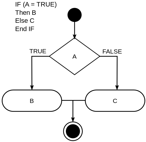
FIGURE 1.1: Control-flow graph representation of an algorithm.
The complexity number is then computed by taking the number of nodes, subtracting the number of edges, and adding twice the number of connected components of this graph. The algorithm is then \(M = E − N + 2P\), where \(M\) is the measure, \(E\) the number of edges, \(N\) the number of nodes and \(2P\) is twice the number of connected components. We will not go deep into this topic, as there are a lot things going on in this computation and you can find much documentation about this online. Please refer to the bibliography for further readings about the theory behind this measurement.
In R, the cyclomatic complexity can be computed using the cyclocomp (Csardi 2016) package.
You can get it from CRAN with:
# Install the {cyclocomp} package
install.packages("cyclocomp")
The cyclocomp package comes with three main functions: cyclocomp(), cyclocomp_package(), and cyclocomp_package_dir().
While developing your application, the one you will be interested in is cyclocomp_package_dir(): building successful shiny apps with the golem framework means you will be building your app as a package (we will get back on that later).
Here is, for example, the cyclomatic complexity of the default golem template (assuming it is located in a golex/ subdirectory):
# Launch the {cyclocomp} package, and compute the
# cyclomatic complexity of "golex",
# A blank {golem} project with one module skeleton
library(cyclocomp)
cyclocomp_package_dir("golex") %>%
  head()
name cyclocomp
1 app_server 1
2 app_ui 1
3 golem_add_external_resources 1
4 run_app 1And the one from another small application:
# Same metric, but for the application
# {tidytuesday201942}, available at
# https://engineering-shiny.org/tidytuesday201942.html
cyclocomp_package("tidytuesday201942") %>%
  head()
name cyclocomp
24 mod_dataviz_ui 8
23 mod_dataviz_server 7
35 rv 6
14 display 4
39 undisplay 4
37 tagRemoveAttributes 3And, finally, the same metric for shiny:
# Computing this metric for the {shiny} package
cyclocomp_package("shiny") %>%
  head()
name cyclocomp
494 untar2 75
115 diagnoseCode 54
389 runApp 50
150 find_panel_info_non_api 37
371 renderTable 37
102 dataTablesJSON 34And, bonus, this cyclocomp_package() function can also be used to retrieve the number of functions inside the package.
As The Clash said, “What are we gonna do now?” You might have heard this saying: “if you copy and paste a piece of code twice, you should write a function”, so you might be tempted to do that. Indeed, splitting code into smaller pieces lowers the local cyclomatic complexity, as smaller functions have lower cyclomatic complexity. But that is just at a local level, and it can be a suboptimal option: having a very large number of functions calling each other can make it harder to navigate through the codebase.
In the end of the day, splitting into smaller functions is not a magic solution because:
- the global complexity of the app is not lowered by splitting things into pieces (just local complexity) and
- The deeper the call stack, the harder it can be to debug.
C. Other measures for code complexity
Complexity can come from other sources: insufficient code coverage, dependencies that break the implementation, relying on old packages, or a lot of other things.
We can use the packageMetrics2 (Csardi 2023) package to get some of these metrics: for example, the number of dependencies, the code coverage, the number of releases and the date of the last one, etc., and the number of lines of code and the cyclomatic complexity.
At the time of writing these lines, the package is not on CRAN and can be installed using the following line of code:
# Installing {packageMetrics2} from GitHub
remotes::install_github("MangoTheCat/packageMetrics2")
This package can now be used to assess the dependencies we use in our application. To do that, let’s create a small function that computes this metric and returns a tibble:
library(packageMetrics2)
# A function to turn the output of the metrics into a data.frame
frame_metric <- function(pkg){
  metrics <- package_metrics(pkg)
  tibble::tibble(
    n = names(metrics),
    val = metrics,
    expl = list_package_metrics()[names(metrics)]
  )
}
And run the metric for golem,
# Using this function with{golem}
frame_metric("golem")
# A tibble: 22 × 3
n val expl
<chr> <chr> <chr>
1 ARR 4 Number of times = i…
2 ATC <NA> Author Test Coverage
3 DWL 82823 Number of Downloads
4 DEP 33 Num of Dependencies
5 DPD 12 Number of Reverse-D…
6 CCP 2.72727272727273 Cyclomatic Complexi…
7 FLE 4.23440285204991 Average number of c…
8 FRE 2019-08-05T14:50:02+00:00 Date of First Relea…
9 LIB 0 Number of library a…
10 LLE 109 Number of code line…
# ℹ 12 more rowsAnd shiny
# Using this function with {shiny}
frame_metric("shiny")
# A tibble: 22 × 3
n val expl
<chr> <chr> <chr>
1 ARR 14 Number of times = i…
2 ATC 46.3623848353278 Author Test Coverage
3 DWL 18122047 Number of Downloads
4 DEP 35 Num of Dependencies
5 DPD 933 Number of Reverse-D…
6 CCP 3.80062794348509 Cyclomatic Complexi…
7 FLE 2.41493883924699 Average number of c…
8 FRE 2012-12-01T07:16:17+00:00 Date of First Relea…
9 LIB 4 Number of library a…
10 LLE 738 Number of code line…
# ℹ 12 more rowsIf you are building your shiny application with golem, you can use the DESCRIPTION file, which contains the list of dependencies, as a starting point to explore these metrics for your dependencies, for example, using desc (Csárdi, Müller, and Hester 2022) or attachment (Rochette and Guyader 2023):
# Get the dependencies from the DESCRIPTION file.
# You can use one of these two functions to list
# the dependencies of your package,
# and compute the metric for each dep
desc::desc_get_deps("golex/DESCRIPTION")
type package version
1 Imports config >= 0.3.1
2 Imports golem >= 0.4.0
3 Imports shiny >= 1.7.4
# See also
attachment::att_from_description("golex/DESCRIPTION")
[1] "config" "golem" "shiny" Some important metrics to watch there are as follow:
- Test coverage: the more the better, as a large code coverage should imply that bugs are more easily caught.
- The number of downloads: a largely downloaded package will likely be less prone to bug, as it will be used by a large user base.
- Number of dependencies: the more a package has dependencies, the more likely it is that at some point it time, something in the dependency graph will break.
- Dates of first publish on CRAN, last publish, and updates: a package actively maintained is a good sign.13
1.2.4 Production-grade software engineering
Complexity is still frowned upon by a lot of developers, notably because it has been seen as something to avoid according to the Unix philosophy. But there are dozens of reasons why an app can become complex: for example, the question your app is answering is quite complex and involves a lot of computation and routines. The resulting app is rather ambitious and implements a lot of features, etc. There is a chance that if you are reading this page, you are working or are planning to work on a complex shiny app. And this is not necessarily a bad thing! shiny apps can definitely be used to implement production-grade 14 software, but production-grade software implies production-grade software engineering. To make your project a success, you need to use tools that reduce the complexity of your app and ensure that your app is resilient to aging.
In other words, production-grade shiny apps require working with a software engineering mindset, which is not always an easy task in the R world: many R developers have learned this language as a tool for doing data analysis, building model, and making statistics; not really as a tool for building software.
The use of R has evolved since its initial version released in 1995, and using this programming language as a tool to build software for production is still a challenge, even 29 years after its first release. And still today, for a lot of R users, the software is still used as an “experimentation tool”, where production quality is one of the least concerns. But the rise of shiny (among other packages) has drastically changed the potential of R as a language for production software engineering: its ease of use is also one of the reasons why the language is now used outside academia, in more “traditional” software engineering teams.
This changing context requires different mindsets, skills, and tools.
With shiny, as we said before, it is quite easy to prototype a simple app, without any “hardcore” software engineering skills. And when we are happy with our little proof of concept, we are tempted to add something new. And another. And another. And without any structured methodology, we are almost certain to reach the cliff of complexity very soon and end up with a codebase that is hardly (if ever) ready to be refactored to be sent to production.
The good news is that building a complex app with R (or with any other language) is not an impossible task. But this requires planning, rigor, and correct engineering. This is what this book is about: how to organize your shiny app in a way that is time and code efficient, and how to use correct engineering to make your app a success.
1.3 What is a successful {shiny} app?
Defining what “successful” means is not an easy task, but we can extract some common patterns when it comes to applications that would be considered successful.
1.3.1 It exists
First of all, an app is successful if it was delivered. In other words, the developer team was able to move from specification to implementation to testing to delivering. This is a very engineering-oriented definition of success, but it is a pragmatic one: an app that never reaches the state of usability is not a successful app, and something along the way has blocked the process of finishing the software.
This condition implies a lot of things, but mostly it implies that the team members were able to organize themselves in an efficient way, so that they were able to work together in making the project a success. Anybody that has already worked on a codebase as a team knows it is not an easy task.
1.3.2 It is accurate
The project is a success if the application was delivered, and if it answers the question it is supposed to answer, or serves the purpose it is supposed to serve. Delivering is not the only thing to keep in mind: you can deliver a working app but it might not work the way it is supposed to work.
Just as before, accuracy means that between the moment the idea appears in someone’s mind and the moment the app is actually ready to be used, everybody was able to work together toward a common goal, and now that this goal is reached, we are also certain that the answers we get from the application are accurate, and that users can rely on the application to make decisions.
1.3.3 It is usable
Being usable means that the app was delivered, it serves the purpose, and it is user-friendly.
Unless you are just coding for the joy of coding, there will always be one or more end users. And if these people cannot use the application because it is too hard to use, too hard to understand, because it is too slow or there is no inherent logic in how the user experience is designed, then it is inappropriate to call the app a success.
1.3.4 It is immortal
Of course, “immortal” is a little bit far-fetched, but when designing the application, you should aim for robustness through the years, by engineering a (theoretically) immortal application.
Planning for the future is a very important component of a successful shiny app project. Once the app is out, it is successful if it can exist in the long run, with all the hazards that this implies: new package versions that could potentially break the codebase, sudden calls for the implementation of new features in the global interface, changing key features of the UI (User Interface) or the back-end, not to mention passing the codebase along to someone who has not worked on the first version, and who is now in charge of developing the next version.15 And this, again, is hard to do without effective planning and efficient engineering.